Projection Perspective

For square-integrable random variables, conditional expectation has a clean geometric interpretation: $\E(X \mid \cG)$ is the orthogonal projection of $X$ onto the closed subspace $L^2(\Omega, \cG, \Pr)$ inside the Hilbert space $L^2(\Omega, \cF, \Pr)$. Two equivalent characterizations make this precise:

• Orthogonality. The residual $X - \E(X \mid \cG)$ is uncorrelated with every $\cG$-measurable square-integrable random variable.
• Minimal distance. Among all $\cG$-measurable square-integrable $Z$, the choice $Z = \E(X \mid \cG)$ minimizes the mean-squared error $\E[(X - Z)^2]$.

Throughout this page, $X$ has $\E[X^2] < \infty$, so $X \in L^2(\Omega, \cF, \Pr)$. The inner product on $L^2$ is $\langle X, Y \rangle = \E[XY]$, and the norm is $\| X \|_2 = \sqrt{\E[X^2]}$. Two zero-mean random variables are uncorrelated iff their inner product (covariance) is zero.

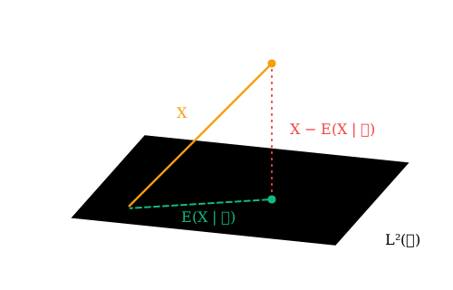
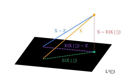
In the drawings below, I use dotted lines to denote something perpendicular to the plane and dashed lines to represent something within the plane.

Orthogonality

Proposition: Orthogonality of the Residual

Statement

Let $X \in L^2(\Omega, \cF, \Pr)$ and let $\cG \subseteq \cF$ be a sub-$\sigma$-field. For every $\cG$-measurable $Y$ with $\E[Y^2] < \infty$,

$$\Cov\!\big( X - \E(X \mid \cG), \; Y \big) \;=\; 0.$$

Equivalently, $X - \E(X \mid \cG)$ is uncorrelated with every $Y \in L^2(\Omega, \cG, \Pr)$. In particular, taking $Y = \E(X \mid \cG)$, the residual is uncorrelated with the projection itself.

Proof

First, $\E[\textcolor{#ef4444}{X - \E(X \mid \cG)}] = \E[X] - \E[\textcolor{#10b981}{\E(X \mid \cG)}] = \E[X] - \E[X] = 0$ by the law of iterated expectations. So

$$\Cov\!\big( X - \E(X \mid \cG), \, Y \big) \;=\; \E\!\big[ Y \big( X - \E(X \mid \cG) \big) \big].$$

It remains to show this expectation is zero. Apply the tower property and condition on $\cG$:

$$\begin{aligned} \E\!\big[ Y \big( X - \E(X \mid \cG) \big) \big] &= \E\!\Big[ \E\!\big( Y (X - \E(X \mid \cG)) \,\big|\, \cG \big) \Big] \\ &= \E\!\Big[ Y \cdot \E\!\big( X - \E(X \mid \cG) \,\big|\, \cG \big) \Big] \\ &= \E\!\big[ Y \cdot \big( \E(X \mid \cG) - \E(X \mid \cG) \big) \big] \\ &= 0. \end{aligned}$$

The second equality uses take-out-what-is-known ($Y$ is $\cG$-measurable, so it pulls out of the inner conditional expectation). The third uses linearity of conditional expectation together with self-measurability of $\E(X \mid \cG)$.

$L^2(\cG)$ is the closed subspace of $\cG$-measurable square-integrable random variables. The projection $\E(X \mid \cG)$ sits in this subspace; the residual $X - \E(X \mid \cG)$ is perpendicular to it.

The reading: covariance is the inner product on the space of mean-zero $L^2$ random variables. The proposition says the residual is orthogonal (uncorrelated) with the whole subspace $L^2(\Omega, \cG, \Pr)$. This is exactly the defining property of an orthogonal projection in Hilbert space.

Minimal distance

Intuition. Any blue line ($X - Z$) is longer than the red perpendicular ($X - \E(X \mid \cG)$). A projection has to be at minimal distance.

Theorem: L²-Minimization

Statement

Let $X \in L^2(\Omega, \cF, \Pr)$. For every $\cG$-measurable $Z$ with $\E[Z^2] < \infty$,

$$\E\!\big[ ( X - \E(X \mid \cG) )^2 \big] \;\le\; \E\!\big[ ( X - Z )^2 \big].$$

Equality holds iff $Z = \E(X \mid \cG)$ a.s. The conditional expectation is the best mean-squared predictor of $X$ among all $\cG$-measurable random variables.

Proof

Decompose $X - Z$ as the sum of the perpendicular $X - \E(X \mid \cG)$ and the in-plane displacement $\E(X \mid \cG) - Z$:

$${X - Z} \;=\; {\big( X - \E(X \mid \cG) \big)} \;+\; {\big( \E(X \mid \cG) - Z \big)}.$$

The first term is the residual; the second is $\cG$-measurable (since both $\E(X \mid \cG)$ and $Z$ are). By orthogonality applied with $Y = \E(X \mid \cG) - Z$, the two terms are uncorrelated. Expanding the square and taking expectation, the cross term vanishes:

$$\begin{aligned} \E\!\big[(X - Z)^2\big] &= \E\!\big[\big( X - \E(X \mid \cG) \big)^2\big] + 2 \, \E\!\big[\big( X - \E(X \mid \cG) \big)\big( \E(X \mid \cG) - Z \big)\big] \\ &\quad + \E\!\big[\big( \E(X \mid \cG) - Z \big)^2\big] \\ &= \E\!\big[\big( X - \E(X \mid \cG) \big)^2\big] + \E\!\big[\big( \E(X \mid \cG) - Z \big)^2\big]. \end{aligned}$$

The purple term is $\ge 0$, with equality iff $\E(X \mid \cG) = Z$ a.s. Dropping it gives the inequality, and the equality case is exactly when $Z = \E(X \mid \cG)$ a.s.

Any alternative $Z \in L^2(\cG)$ produces a longer line $X - Z$ than the perpendicular $X - \E(X \mid \cG)$. The Pythagorean identity $\|X - Z\|_2^2 = \|X - \E(X \mid \cG)\|_2^2 + \|\E(X \mid \cG) - Z\|_2^2$ is the algebraic content of the picture.

Putting the pieces together

The two characterizations (orthogonality, minimal distance) are equivalent statements of the Hilbert-space projection theorem specialized to the closed subspace $L^2(\Omega, \cG, \Pr) \subseteq L^2(\Omega, \cF, \Pr)$. For any closed subspace $M$ of a Hilbert space $H$ and any $X \in H$:

• A unique $\hat X \in M$ minimizes $\| X - Z \|$ over $Z \in M$.
• This $\hat X$ is characterized by $X - \hat X \perp M$.

Conditional expectation realizes this projection concretely: $\hat X = \E(X \mid \cG)$. The construction we gave via Radon-Nikodym handles all integrable $X$ (not just $X \in L^2$), but on the $L^2$ subset it coincides with the projection, and most intuition transfers from the geometric picture.

A few corollaries that fall out immediately:

• Variance decomposition. Taking $Z = \E[X]$ (the trivial-$\sigma$-field projection) in the Pythagorean identity gives

$$\Var(X) \;=\; \E[\Var(X \mid \cG)] + \Var(\E(X \mid \cG)),$$

the law of total variance: unconditional variance splits into the conditional-variance average plus the variance of the conditional mean.

• Best linear prediction. Restricting $\cG$ to be the $\sigma$-field generated by a finite collection $\{Y_1, \ldots, Y_k\}$ and further restricting to linear combinations of the $Y_i$ recovers ordinary least-squares regression. The conditional expectation is the best predictor; OLS is the best linear predictor.

• Idempotence. Projection is idempotent: applying $\E(\cdot \mid \cG)$ twice gives the same answer, which is the tower property restricted to $L^2$.